Excel Article

Excel Tables (Part 2) - Creating an Excel Table

It is possible to create an Excel Table on a blank worksheet, and then rename the columns, but I would strongly recommend that you start with a plain table first, even if it has no data in it. Figure out what columns you are going to need, their naming and what is the best order for and finally convert it to an Excel Table

If you can, group columns that will require user input together, and try and keep them to the left hand side of the table, with calculated results more to the right hand side.

One rule with Excel Tables is that column names must be unique. Also I would suggest that column names start with a letter, so that you cannot accidentally add them in to get an erroneous total.

As a demonstration example we will build an Excel Table to manage your current account.

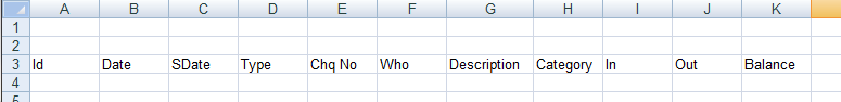
In a new Workbook, add the following column names

• Id – We will explain this column in a future article
• Date – Date of transaction, for example when you wrote a cheque out
• SDate – Date item appears on the bank statement
• Type – Type of transaction, for example Standing Order, Direct Debit etc
• Chq No – Cheque number
• Who – The person who has paid you or who you are paying
• Description – What you purchased or why you received a payment
• Category – Useful if you want to analyse your expenditure
• In – Payments in
• Out – Payments out
• Balance – A running total

You should end up with something like this.

You may decide you don’t need all these columns, and that’s fine.

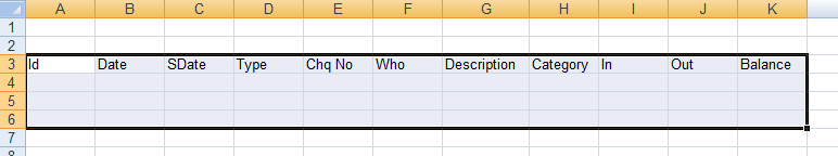
Now we have our basic plain table, select the columns plus a few rows underneath, like this.

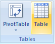
Then go to the insert menu and click on the Table icon.

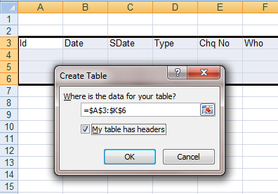
When the dialog appears, make sure the "My table has headers" tick box is ticked.

In the Table Tools design menu, enter a name for your table. This is optional but good practice.

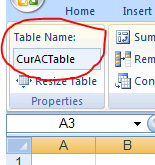
A tip here is to add Table to the end of the name. It will make them easier to spot when looking through named items. In the picture above you can see them by clicking on the small triangle to the right of the A3.

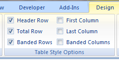
While still in the Table Tools Design menu, tick the "Total Row" check box in Table Style Options.

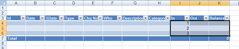
This is the resulting Excel Table.

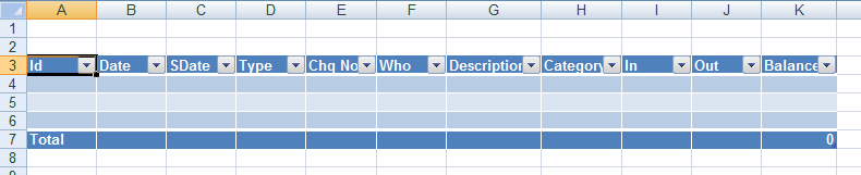
From this we can see the parts that make up an Excel Table

• In row 3 we have the header row
• In rows 4, 5 and 6 we have the data rows
• And in row 7 we have the total row

We take a deeper look at formatting Excel Tables in a future article, but let's highlight one key aspect now.

In the "In" column we will enter some numeric values

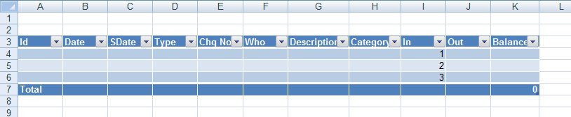
However the format of these numbers is not how I like for money.

To change this, select the money related columns, and the key point here is to select all the data rows.

Then right click and choose Format Cells. In the dialog, choose your preferred number format for currency

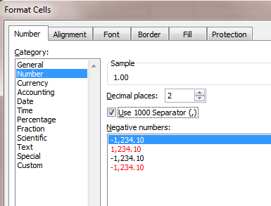
In my case I want two decimal places, a comma separator for thousands, and a plain number format not currency format – I dislike having the currency symbol in every cell – but that is a personal preference. This is the result with a bit more dummy data added.

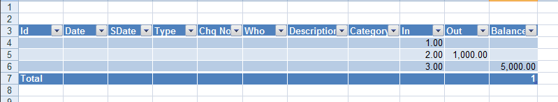
Because we selected all the data rows, the numeric format will automatically be used when we add or insert more data rows into the table. It is easier to apply the formatting at this point rather than when the table has hundreds of rows.

In the next article we will look at Table References before returning to our current account table

Screen shots created in Excel 2007 on Windows 7